Sage Bionetworks NF-OSI Research: DRUID analysis of JHU Biobank data

Publicly available data from JHU Biobank

We used the publicly available JHU Biobank RNASeq data stored in project : syn20812185 for this analysis.

We then used TMM normalization to prepare the dataset for differential gene expression analysis.

Differential gene expression analysis in samples:

We used limma-edgeR based analysis to find differentially expressed genes in the TMM normalized dataset.

A point to note:

All MPNST samples except one are males while all PNF samples except one are femmales. So there may be a sex related effect on the analysis that we dont have a good way to mitigate.
The number of MPNST samples are extremely limited (n=4), so these results should be evaluated with more samples when possible

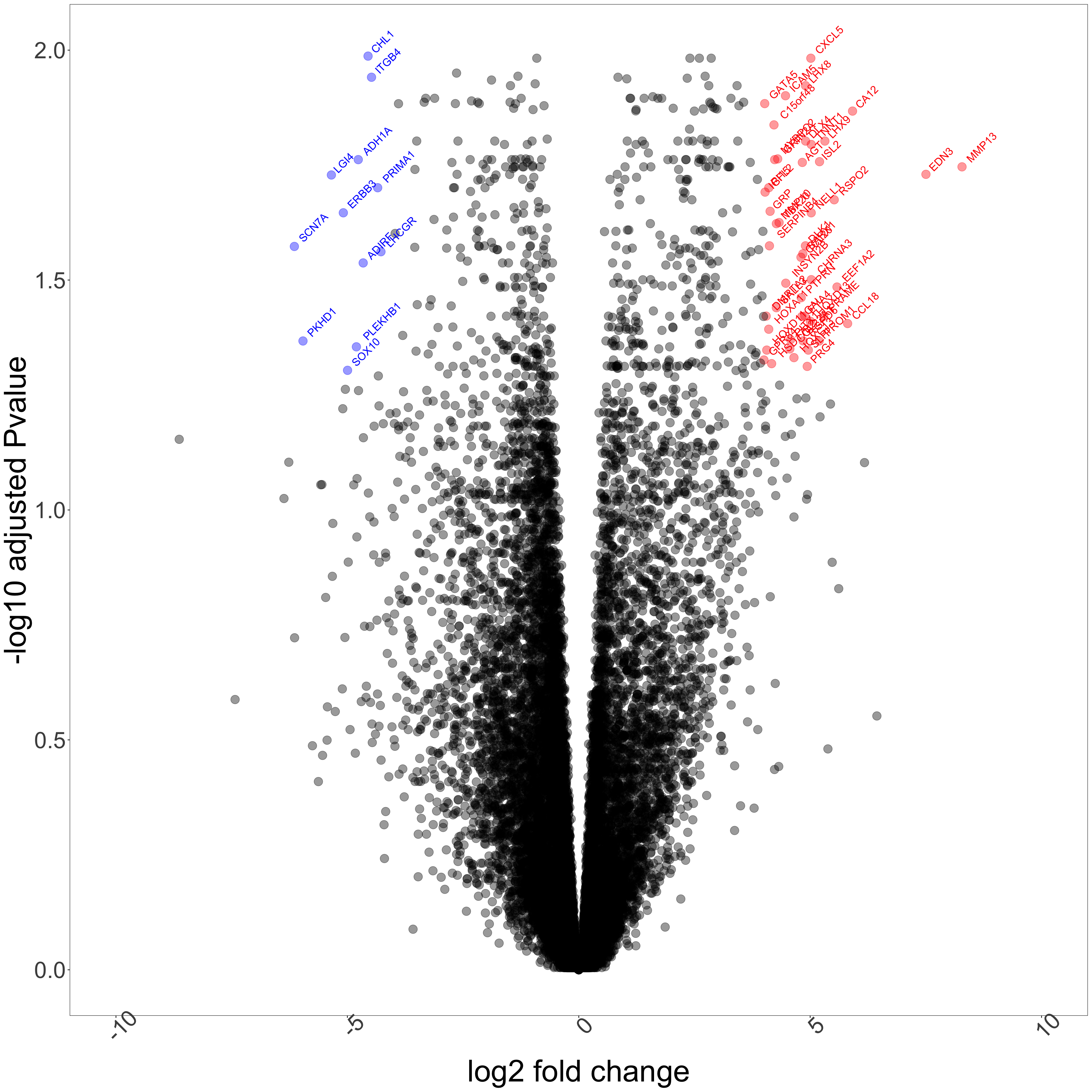
The plot below shows genes that are significantly overexpressed in MPNST compared to PNF (logFC > 4) in red. The dots in blue refer to genes that are significantly underexpressed in MPNST compared to PNF (logFC < -4). The thresholds of fold change have been arbitrarily chosen for ease of visualization in the volcano plot shown below.

Differential expression of genes in MPNST and pNF tumor types. Above shows a volcano plot highlighting significantly upregulated genes in red and downregulated genes in blue

Figure 1: Differential expression of genes in MPNST and pNF tumor types. Above shows a volcano plot highlighting significantly upregulated genes in red and downregulated genes in blue

Predicting drug candidates based on significant DEGs using DRUID:

We then took the subset of genes that were significantly differentially expressed between MPNST and pNF tumor types and used DRUID to enrich candidate drugs to revert the MPNST phenotype to pNF phenotype. We did this using the following steps:

# Select the significantly differentially expressed genes from DEG analysis
druid_dge <- MPNSTvsPNF %>% 
  dplyr::select(c("logFC","adj.P.Val")) %>% 
  dplyr::filter(MPNSTvsPNF$adj.P.Val < 0.05)
  
# Make query matrix for DRUID
query_matrix <- as.matrix(druid_dge)

# Convert the gene names to entrez ids
geneSymbols <- AnnotationDbi::mapIds(org.Hs.eg.db, 
                                     keys=rownames(query_matrix), 
                                     column=c("ENTREZID"), 
                                     keytype="SYMBOL", 
                                     multiVals = "first") %>% as.data.frame()
#head(geneSymbols)
entrez_ids <- geneSymbols$.

# # Run Druid with only significant genes (adj_p_val < 0.05) and save output
# sig_genes_druid <- concoct(dge_matrix = query_matrix, 
#                            num_random = 10000, 
#                            druid_direction = "neg", 
#                            fold_thr = 0.5, 
#                            pvalue_thr = 0.05, 
#                            entrez = entrez_ids)
# sig_genes_druid_ordered <- sig_genes_druid[order(sig_genes_druid$druid_score, decreasing = TRUE),]
# #head(sig_genes_druid_ordered)
# 
# save(sig_genes_druid_ordered, file = "./sig_genes_druid_mpnst_pnf.RData")

load("./sig_genes_druid_mpnst_pnf.RData")


sig_genes_druid_ordered %>% 
  dplyr::filter(., druid_score > 5) %>% 
  ggplot() + 
  geom_point(aes(x = drug_name, y = cosine_similarity, color = cell_line), alpha = 0.5) + 
  facet_grid(. ~ cell_line, scales = "free") + 
  theme_bw() + 
  theme(axis.text.x = element_text(angle = 45))

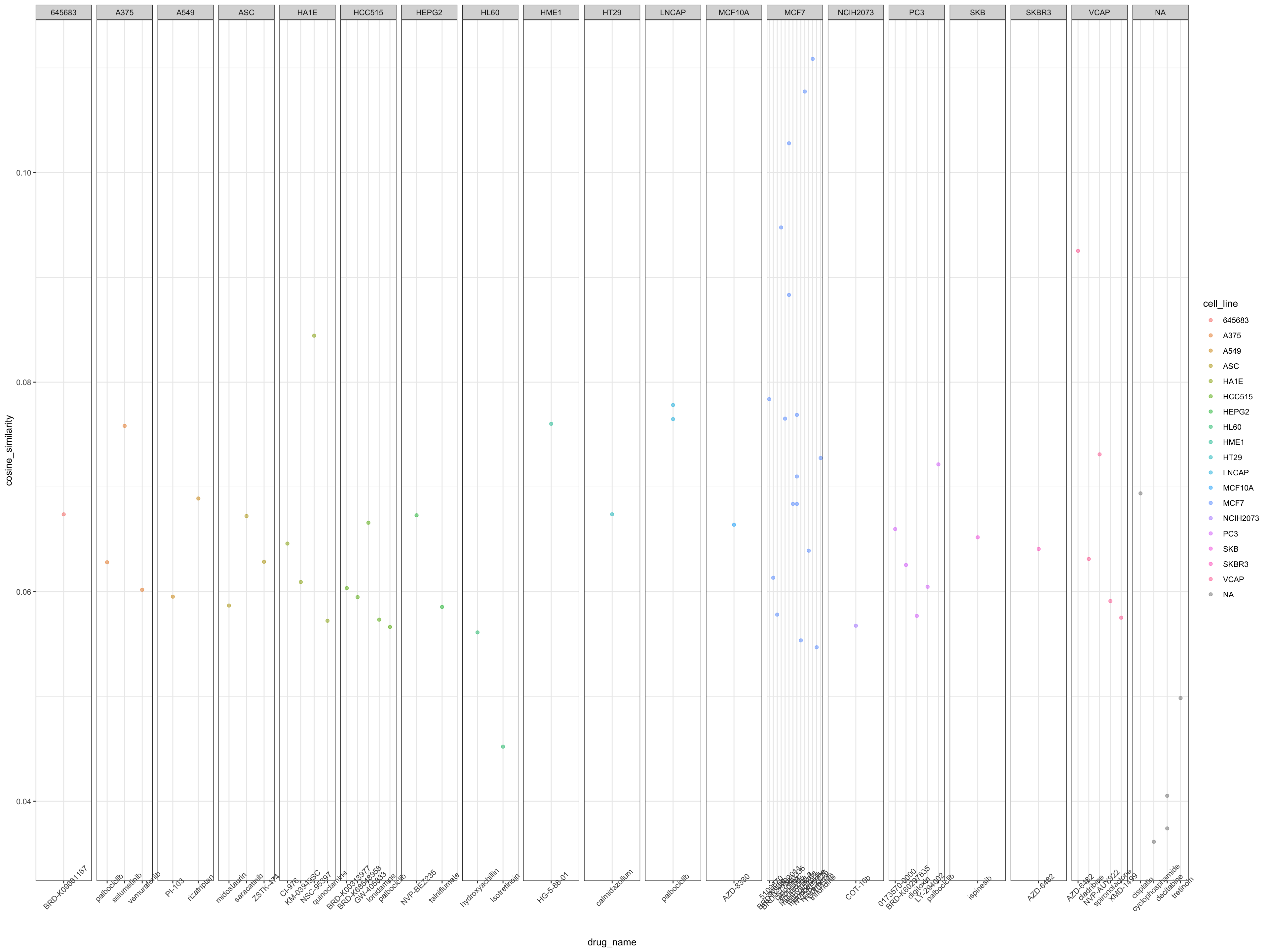
Figure 2: DRUID predictions for significant DEGs

The table below lists all the drugs that were recommended as promising candidates using the DRUID analysis. A higher DRUID score (scale from 0-6) would mean a higher recommendation for the drug compound.

Distill is a publication format for scientific and technical writing, native to the web.

Learn more about using Distill for R Markdown at https://rstudio.github.io/distill.